04-多层感知机

Posted Jan 29, 2025 Updated Aug 5, 2025

By hhhi21g

15 min read

04-多层感知机

4.1 多层感知机

多层感知机概念

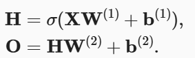
将许多全连接层堆叠在一起，每一层都输出到上面的层，直到生成最后的输出。这种架构通常称为多层感知机，通常缩写为MLP。

为了发挥多层架构的潜力，需要: 在仿射变换之后对每个隐藏单元应用非线性的激活函数，如下：

激活函数

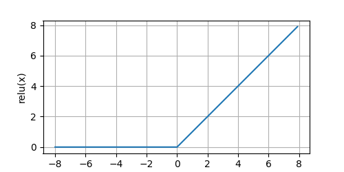
ReLU函数：

使用实例：

  
# ReLU函数
x = torch.arange(-8.0, 8.0, 0.1, requires_grad=True)
y = torch.relu(x)
d2l.plot(x.detach(), y.detach(), 'x', 'relu(x)', figsize=(5, 2.5))
d2l.plt.show()

  
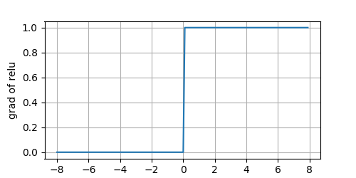
y.backward(torch.ones_like(x), retain_graph=True)  # 保留计算图，在后续反向传播中继续使用这个图
d2l.plot(x.detach(), x.grad, 'x', 'grad of relu', figsize=(5, 2.5))
d2l.plt.show()

ReLU函数及其导数图像：

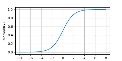
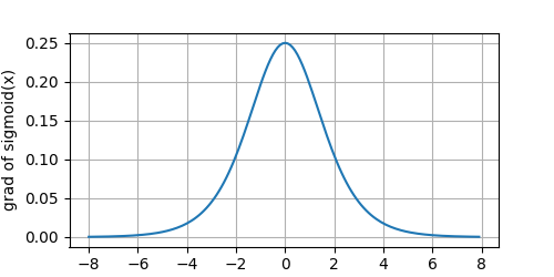
sigmoid函数：

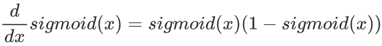
函数及其导数图像：

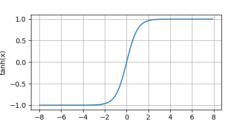
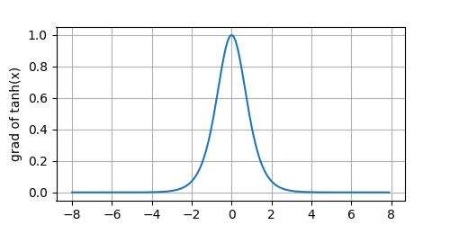
tanh函数：

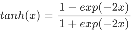
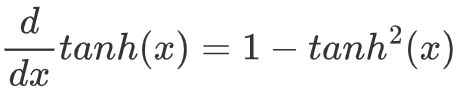
函数及其导数图像：

4.2 多层感知机的从零开始实现

base:

  
import torch
from torch import nn
from d2l import torch as d2l

batch_size = 256
train_iter, test_iter = d2l.load_data_fashion_mnist(batch_size)

初始化模型参数：

  
num_inputs, num_outputs, num_hiddens = 784, 10, 256

w1 = nn.Parameter(
    torch.randn(num_inputs, num_hiddens, requires_grad=True) * 0.01
)
b1 = nn.Parameter(torch.zeros(num_hiddens, requires_grad=True))
w2 = nn.Parameter(
    torch.randn(num_hiddens, num_outputs, requires_grad=True) * 0.01
)
b2 = nn.Parameter(torch.zeros(num_outputs, requires_grad=True))

params = [w1, b1, w2, b2]

激活函数：

  
def relu(X):
    a = torch.zeros_like(X)
    return torch.max(X, a)

模型：

  
def net(X):
    X = X.reshape((-1, num_inputs))
    H = relu(X @ w1 + b1)
    return (H @ w2 + b2)  # @表示矩阵乘法

# 损失函数
loss = nn.CrossEntropyLoss(reduction='none')

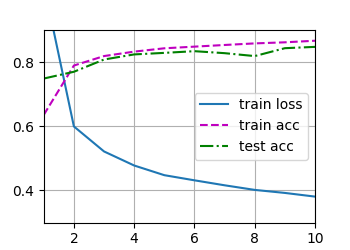
训练：

  
num_epochs, lr = 10, 0.1
updater = torch.optim.SGD(params, lr=lr)
d2l.train_ch3(net, train_iter, test_iter, loss, num_epochs, updater)
d2l.plt.show()

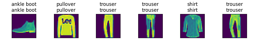
d2l.predict_ch3(net, test_iter)
d2l.plt.figure(figsize=(10,6))  # 为了标签文本显示完整
d2l.plt.show()

结果：

4.3 多层感知机的简洁实现

模型：

  
net = nn.Sequential(nn.Flatten(),
                    nn.Linear(784, 256),
                    nn.ReLU(),
                    nn.Linear(256, 10))

  
def init_weights(m):
    if type(m) == nn.Linear:
        nn.init.normal_(m.weight, std=0.01)

net.apply(init_weights)

训练：

  
batch_size, lr, num_epochs = 256, 0.1, 10
loss = nn.CrossEntropyLoss(reduction='none')
trainer = torch.optim.SGD(net.parameters(), lr=lr)

train_iter, test_iter = d2l.load_data_fashion_mnist(batch_size)
d2l.train_ch3(net,train_iter, test_iter, loss,num_epochs, trainer)
d2l.plt.show()

4.4 模型选择、欠拟合和过拟合

一些概念

过拟合：将模型在训练数据上拟合的比在潜在分布中更接近的现象
用于对抗过拟合的技术称为正则化
训练误差：模型在训练数据集上计算得到的误差
泛化误差：模型应用在同样从原始样本的分布中抽取的无限多数据样本时，模型误差的期望
独立同分布假设：假设训练数据和测试数据都是从相同的分布中独立提取得到
K折交叉验证：原始训练数据被分为K个不重叠的子集，然后执行K次模型训练和验证，每次在K-1个子集上进行训练，并在剩余的一个子集（在该轮中没有用于训练的子集）上进行验证，最后通过对K次实验的结果取平均来估计训练和验证误差

几个倾向于影响模型泛化的因素：

可调整参数的数量。当可调整参数的数量（有时称为自由度）很大时，模型往往更容易过拟合。
参数采用的值。当权重的取值范围较大时，模型可能更容易过拟合。
训练样本的数量。即使模型很简单，也很容易过拟合只包含一两个样本的数据集。而过拟合一个有数百万个样本的数据集则需要一个极其灵活的模型。

区分欠拟合与过拟合：

欠拟合：训练误差和验证误差都很严重，但它们之间仅有一点差距，如果模型不能降低训练误差可能意味着模型过于简单；此外，由于训练和验证之间的泛化误差很小，有理由相信可以用一个更复杂的模型降低训练误差。

过拟合：训练误差明显低于验证误差

最好的预测模型在训练数据上的表现往往比验证数据上好得多，最终我们通常更关心验证误差，而不是训练误差和验证误差之间的差距。

使用实例

保存至d2l:

  
def evaluate_loss(net, data_iter, loss):  # @save
    """评估给定数据集上模型的损失"""
    metric = d2l.Accumulator(2)  # 损失的总和,样本数量
    for X, y in data_iter:
        out = net(X)
        y = y.reshape(out.shape)
        l = loss(out, y)
        metric.add(l.sum(), l.numel())
    return metric[0] / metric[1]

  
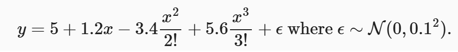
# 通常希望避免非常大的梯度值或损失值,因此除以阶乘
max_degree = 20  # 多项式的最大阶数
n_train, n_test = 100, 100  # 训练和测试数据集的大小
true_w = np.zeros(max_degree)
true_w[0:4] = np.array([5, 1.2, -3.4, 5.6])

features = np.random.normal(size=(n_train + n_test, 1))
np.random.shuffle(features)
poly_features = np.power(features, np.arange(max_degree).reshape(1, -1))
for i in range(max_degree):
    poly_features[:, i] /= math.gamma(i + 1)  # gamma(n) = (n - 1)!
labels = np.dot(poly_features, true_w)
labels += np.random.normal(scale=0.1, size=labels.shape)

# NumPy ndarray转换为tensor
true_w, features, poly_features, labels = [torch.tensor(x, dtype=
torch.float32) for x in [true_w, features, poly_features, labels]]

  
def train(train_features, test_features, train_labels, test_labels,
          num_epochs=400):
    loss = nn.MSELoss(reduction='none')
    input_shape = train_features.shape[-1]
    # 不设置偏置，因为我们已经在多项式中实现了它
    net = nn.Sequential(nn.Linear(input_shape, 1, bias=False))
    batch_size = min(10, train_labels.shape[0])
    train_iter = d2l.load_array((train_features, train_labels.reshape(-1, 1)),
                                batch_size)
    test_iter = d2l.load_array((test_features, test_labels.reshape(-1, 1)),
                               batch_size, is_train=False)
    trainer = torch.optim.SGD(net.parameters(), lr=0.01)
    animator = d2l.Animator(xlabel='epoch', ylabel='loss', yscale='log',
                            xlim=[1, num_epochs], ylim=[1e-3, 1e2],
                            legend=['train', 'test'])
    for epoch in range(num_epochs):
        d2l.train_epoch_ch3(net, train_iter, loss, trainer)
        if epoch == 0 or (epoch + 1) % 20 == 0:
            animator.add(epoch + 1, (evaluate_loss(net, train_iter, loss),
                                     evaluate_loss(net, test_iter, loss)))
    print('weight:', net[0].weight.data.numpy())

绘图：

  
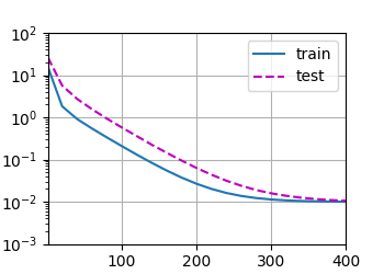
# 从多项式特征中选择前4个维度，即1,x,x^2/2!,x^3/3!，正常
train(poly_features[:n_train, :4], poly_features[n_train:, :4],
      labels[:n_train], labels[n_train:])
d2l.plt.show()

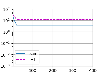
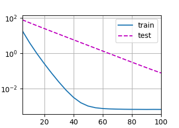
# 从多项式特征中选择前2个维度，即1和x，欠拟合
train(poly_features[:n_train, :2], poly_features[n_train:, :2],
      labels[:n_train], labels[n_train:])
d2l.plt.show()

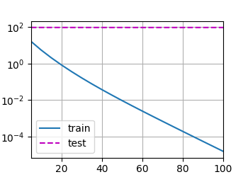
# 从多项式特征中选取所有维度，过拟合
train(poly_features[:n_train, :], poly_features[n_train:, :],
      labels[:n_train], labels[n_train:], num_epochs=1500)
d2l.plt.show()

<img src="https://hhhi21g.github.io/assets/img/deepLearning/pic443.png" alt="alt text" style="zoom:75%;" />

</p>

4.5 权重衰减

最广泛使用的正则化的技术之一，它通常也被称为L₂正则化；这项技术通过函数与0的距离来衡量函数的复杂度。

正则化是处理过拟合的常用方法：在训练集的损失函数中加入惩罚项，以降低学习到的模型的复杂度

线性回归的损失：

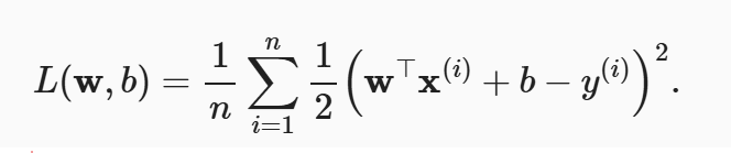
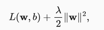
为了惩罚权重向量的大小，必须以某种方式在损失函数中添加||w||², 通过正则化常数λ来描述这种权衡，这是一个非负超参数，使用验证数据拟合：

L₂正则化回归的小批量随机梯度下降更新如下式：

使用L₂而不是L₁:

L₂范数对权重向量的大分量施加了巨大的惩罚，这使得我们的学习算法偏向于在大量特征上均匀分布权重的模型；在实践中，这可能使它们对单个变量中的观测误差更加稳定。相比之下，L₁惩罚会导致模型将权重集中在一小部分特征上，而将其他权重清除为0，这成为特征选择。

从零开始实现

  
import torch
from torch import nn
from d2l import torch as d2l

n_train,n_test,num_inputs,batch_size = 20,100,200,5
true_w,true_b = torch.ones((num_inputs,1))*0.01,0.05

train_data = d2l.synthetic_data(true_w,true_b,n_train)
train_iter = d2l.load_array(train_data,batch_size)

test_data = d2l.synthetic_data(true_w,true_b,n_test)
test_iter = d2l.load_array(test_data,batch_size,is_train=False)

# 从零开始实现权重衰退
# 随机初始化模型参数
def init_params():
    w = torch.normal(0,1,size=(num_inputs,1),requires_grad=True)
    b = torch.zeros(1,requires_grad=True)
    return [w,b]

# 定义L2范数惩罚
def l2_penalty(w):
    return torch.sum(w.pow(2))/2

def train(lambd):
    w,b = init_params()
    net,loss = lambda X:d2l.linreg(X,w,b),d2l.squared_loss
    num_epochs,lr = 100,0.003
    animator = d2l.Animator(xlabel='epochs',ylabel='loss',yscale='log',
                            xlim=[5,num_epochs],legend=['train','test'])
    for epoch in range(num_epochs):
        for X,y in train_iter:
            l = loss(net(X),y)+lambd*l2_penalty(w)
            l.sum().backward()
            d2l.sgd([w,b],lr,batch_size)
        if(epoch+1)%5==0:
            animator.add(epoch+1,(d2l.evaluate_loss(net,train_iter,loss),
                                  (d2l.evaluate_loss(net,test_iter,loss))))
    print("w的L2范数是:",torch.norm(w).item());

train(lambd = 0)
train(lambd = 3)
d2l.plt.show()

结果：

这里训练误差增大，但测试误差减小，正是期望从正则化中得到的效果。

简洁实现

  
def train_concise(wd):
    net = nn.Sequential(nn.Linear(num_inputs,1))
    for param in net.parameters():
        param.data.normal_()
    loss = nn.MSELoss(reduction='none')
    num_epochs,lr = 100,0.003
    # 偏置参数没有衰减
    trainer = torch.optim.SGD([
        {"params":net[0].weight,'weight_decay':wd},
        {"params":net[0].bias}
    ], lr = lr)
    animator = d2l.Animator(xlabel='epochs', ylabel='loss', yscale='log',
                            xlim=[5, num_epochs], legend=['train', 'test'])
    for epoch in range(num_epochs):
        for X, y in train_iter:
            trainer.zero_grad()
            l = loss(net(X), y)
            l.mean().backward()
            trainer.step()
        if (epoch + 1) % 5 == 0:
            animator.add(epoch + 1,
                         (d2l.evaluate_loss(net, train_iter, loss),
                          d2l.evaluate_loss(net, test_iter, loss)))
    print('w的L2范数：', net[0].weight.norm().item())

train_concise(0)
train_concise(3)
d2l.plt.show()

4.6 暂退法(Dropout)

在训练过程中，建议在计算后续层之前向网络的每一层注入噪声。因为当训练一个有多层的深层网络时，注入噪声只会在输入-输出映射上增强平滑性。这个想法被称为暂退法。

从表面上看是在训练过程中丢弃一些神经元。在整个训练过程的每一次迭代中，标准暂退法包括在计算下一层之前将当前层的一些节点置零。

每个中间活性值h以暂退概率p由随机变量h’替换：

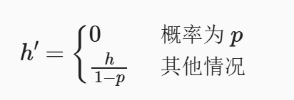
根据此模型的设计，其期望值保持不变，即E[h’] = h。

从零开始实现

单层的暂退法函数：

  
def dropout_layer(X, dropout):
    assert 0 <= dropout <= 1
    # 所有元素都被丢弃
    if dropout == 1:
        return torch.zeros_like(X)
    # 所有元素都被保留
    if dropout == 0:
        return X
    mask = (torch.rand(X.shape) > dropout).float()
    return mask * X / (1.0 - dropout)


X = torch.arange(16, dtype=torch.float32).reshape((2, 8))
print(X)
print(dropout_layer(X, 0.))
print(dropout_layer(X, 0.5))
print(dropout_layer(X, 1.))

tensor([[ 0., 1., 2., 3., 4., 5., 6., 7.], [ 8., 9., 10., 11., 12., 13., 14., 15.]])
tensor([[ 0., 1., 2., 3., 4., 5., 6., 7.], [ 8., 9., 10., 11., 12., 13., 14., 15.]])
tensor([[ 0., 0., 4., 0., 8., 0., 12., 0.], [ 0., 0., 20., 22., 24., 0., 0., 30.]])
tensor([[0., 0., 0., 0., 0., 0., 0., 0.], [0., 0., 0., 0., 0., 0., 0., 0.]])

定义模型：

  
num_inputs, num_outputs, num_hiddens1, num_hiddens2 = 784, 10, 256, 256

# 常见技巧为：靠近输入层的地方设置较低的暂退概率
dropout1, dropout2 = 0.2, 0.5

class Net(nn.Module):
    def __init__(self, num_inputs, num_outputs, num_hiddens1, num_hiddens2,
                 is_training=True):
        super(Net, self).__init__()
        self.num_inputs = num_inputs
        self.training = is_training
        self.lin1 = nn.Linear(num_inputs, num_hiddens1)
        self.lin2 = nn.Linear(num_hiddens1, num_hiddens2)
        self.lin3 = nn.Linear(num_hiddens2, num_outputs)
        self.relu = nn.ReLU()

    def forward(self, X):
        H1 = self.relu(self.lin1(X.reshape(-1, self.num_inputs)))
        # 只有在训练模型时才使用dropout
        if self.training == True:
            # 在第一个全连接层之后添加一个dropout层
            H1 = dropout_layer(H1, dropout1)
        H2 = self.relu(self.lin2(H1))
        if self.training == True:
            H2 = dropout_layer(H2, dropout2)
        out = self.lin3(H2)
        return out

net = Net(num_inputs, num_outputs, num_hiddens1, num_hiddens2)

训练和测试：

  
num_epochs, lr, batch_size = 10, 0.5, 256
loss = nn.CrossEntropyLoss(reduction='none')
train_iter, test_iter = d2l.load_data_fashion_mnist(batch_size)
trainer = torch.optim.SGD(net.parameters(), lr=lr)
d2l.train_ch3(net, train_iter, test_iter, loss, num_epochs, trainer)
d2l.plt.show()

简洁实现

  
net = nn.Sequential(nn.Flatten(),
                    nn.Linear(784,256),
                    nn.ReLU(),
                    nn.Dropout(dropout1),
                    nn.Linear(256,256),
                    nn.ReLU(),
                    nn.Dropout(dropout2),
                    nn.Linear(256,10))

def init_weights(m):
    if type(m) == nn.Linear():
        nn.init.normal_(m.weight,std=0.01)

net.apply(init_weights)
trainer = torch.optim.SGD(net.parameters(), lr=lr)
d2l.train_ch3(net, train_iter, test_iter, loss, num_epochs, trainer)
d2l.plt.show()

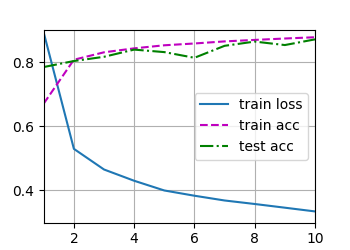
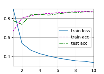
上为从零开始，下为简洁实现

深度学习

This post is licensed under CC BY 4.0 by the author.

4.1 多层感知机

多层感知机概念

激活函数

4.2 多层感知机的从零开始实现

4.3 多层感知机的简洁实现

4.4 模型选择、欠拟合和过拟合

一些概念

使用实例

4.5 权重衰减

从零开始实现

简洁实现

4.6 暂退法(Dropout)

从零开始实现

简洁实现

Trending Tags