03-线性神经网络
3.1 线性回归😂
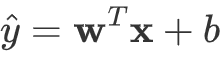
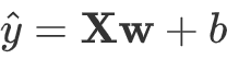
线性模型
向量x: 所有特征
向量w: 所有权重 (向量为垂直方向排列, 点积)
矩阵X: 每一行是一个样本,每一列是一种特征(矩阵-向量乘法)
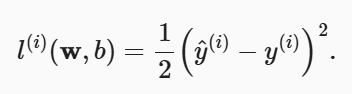
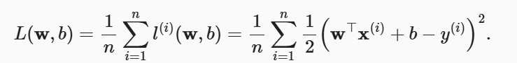
损失函数
平方误差(0.5使得求导后常数系数为1):
损失均值:
随机梯度下降
| ß: 随机取样的一个小批量,由固定数量的训练样本组成( | ß | :批量大小) |
ŋ: 学习率
通常手动预先指定,这些可以调整但不在训练过程中更新的参数称为超参数 ,调参是选择超参数的过程,训练迭代结果是在独立的验证数据集上评估得到的。
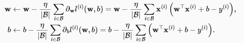
公式后面为误差均值,原值 - 学习率 * 误差均值 以修正
泛化:找到一组参数,能够在我们从未见过的数据上实现较低的损失
矢量化加速
#@save类Timer
start: # 启动计时器
stop: # 停止计时器并将时间记录在列表中
avg: # 返回平均时间
sum: # 返回时间总和
cumsum: # 返回累计时间
使用实例:
1
2
3
4
5
6
7
n = 10000
a = torch.ones([n])
b = torch.ones([n])

timer = Timer()
d = a + b
print(f'{timer.stop():.5f} sec')  # 矢量化代码通常会带来数量级的加速
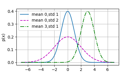
正态分布绘图实例
概率密度函数:
1
2
3
def normal(x, mu, sigma):
    p = 1 / math.sqrt(2 * math.pi * sigma ** 2)
    return p * np.exp(-(x - mu) ** 2 / (2 * sigma ** 2))
可视化:
1
2
3
4
5
6
7
x = np.arange(-7, 7, 0.01)

params = [(0, 1), (0, 2), (3, 1)]
d2l.plot(x, [normal(x, mu, sigma) for mu, sigma in params], xlabel='x',
         ylabel='p(x)', figsize=(4.5, 2.5),
         legend=[f'mean {mu},std {sigma}' for mu, sigma in params])
plt.show()
线性神经图
神经网络的层数:计算层数时不考虑输入层
全连接层(稠密层):每个输入都与每个输出相连
3.2 线性回归的从零开始实现
保存至d2l的函数:
1
2
3
4
5
6
# 生成y = Xw + b + 噪声
def synthetic_data(w, b, num_examples):  # @save
    X = torch.normal(0, 1, (num_examples, len(w)))
    y = torch.matmul(X, w) + b
    y += torch.normal(0, 0.01, y.shape)
    return X, y.reshape((-1, 1))
1
2
3
# 线性回归模型
def linreg(X, w, b):  # @save
    return torch.matmul(X, w) + b
1
2
3
# 损失函数
def squared_loss(y_hat, y):  # @save
    return (y_hat - y.reshape(y_hat.shape)) ** 2 / 2
1
2
3
4
5
6
# 小批量随机梯度下降
def sgd(params, lr, batch_size):  # @save
    with torch.no_grad():  # 不进行梯度追踪,节省内存和计算资源
        for param in params:
            param -= lr * param.grad / batch_size
            param.grad.zero_()
绘制散点图实例:
1
2
3
d2l.set_figsize()
d2l.plt.scatter(features[:, (1)].detach().numpy(), labels.detach().numpy(), 1)
plt.show()
随机读取小批量样本实例:
1
2
3
4
5
6
7
8
9
def data_iter(batch_size, features, labels):
    num_examples = len(features)
    indices = list(range(num_examples))
    random.shuffle(indices)
    for i in range(0, num_examples, batch_size):
        batch_indices = torch.tensor(
            indices[i:min(i + batch_size, num_examples)]
        )
        yield features[batch_indices], labels[batch_indices]
训练实例:
1
2
3
4
5
6
7
8
9
10
11
12
13
lr = 0.03
num_epochs = 3
net = linreg
loss = squared_loss

for epoch in range(num_epochs):
    for X, y in data_iter(batch_size, features, labels):
        l = loss(net(X, w, b), y)  # l的形状为[batch_size,1],非标量
        l.sum().backward()
        sgd([w, b], lr, batch_size)
    with torch.no_grad():
        train_l = loss(net(features, w, b), labels)
        print(f'epoch {epoch + 1}, loss {float(train_l.mean()):f}')
3.3 线性回归的简洁实现
import:
1
2
3
import torch
from d2l import torch as d2l
from torch.utils import data
保存至d2l的函数:
1
2
3
4
# 构造一个pytorch数据迭代器
def load_array(data_arrays, batch_size, is_train=True):  # @save
    dataset = data.TensorDataset(*data_arrays)  # 将输入的张量包装成一个数据集对象
    return data.DataLoader(dataset, batch_size, shuffle=is_train)
生成数据集
1
2
3
true_w = torch.tensor([2, -3.4])
true_b = 4.2
features, labels = d2l.synthetic_data(true_w, true_b, 1000)
读取数据集
1
2
batch_size = 10
data_iter = load_array((features, labels), batch_size)
1
2
3
print(next(iter(data_iter)))  # iter()显式地创建一个迭代器
# iter()函数返回的是一个迭代器,本身并不返回数据;
# 只有调用next()时,迭代器才会开始迭代并返回数据
[tensor([[-0.4443, -1.2958], [-0.7646, 0.6442], [ 0.0836, -1.3110], [-0.4851, -1.1598], [ 0.4348, -0.1553], [ 0.2450, -0.4867], [ 0.2895, 1.1791], [-0.3936, 0.7068], [ 0.6898, 0.2431], [ 1.4839, -0.4528]]),
tensor([[7.7131], [0.4788], [8.8145], [7.1686], [5.6042], [6.3388], [0.7815], [1.0104], [4.7435], [8.7051]])]
定义模型
1
2
from torch import nn
net = nn.Sequential(nn.Linear(2, 1))
初始化模型参数
1
2
net[0].weight.data.normal_(0, 0.01)
net[0].bias.data.fill_(0)
定义损失参数
1
2
# MSELoss类,也称平方L2范数, 默认情况返回所有样本损失的平均值
loss = nn.MSELoss()
定义优化算法
1
trainer = torch.optim.SGD(net.parameters(), lr=0.03)
训练
1
2
3
4
5
6
7
8
9
10
11
num_epochs = 3
for epoch in range(num_epochs):
    for X, y in data_iter:
        l = loss(net(X), y)
        trainer.zero_grad()
        l.backward()
        trainer.step()
        # 根据已经计算的梯度更新模型的参数
        # 根据指定的优化算法(SGD,Adam等)调整参数
    l = loss(net(features), labels)
    print(f'epoch {epoch + 1}, loss {l:f}')
epoch 1, loss 0.000246
epoch 2, loss 0.000102
epoch 3, loss 0.0001011 2 3 4 5
# 比较生成数据集的真实参数和通过有限数据训练获得的模型参数 w = net[0].weight.data print('w的估计误差:',true_w - w.reshape(true_w.shape)) b = net[0].bias.data print('b的估计误差:',true_b - b)
w的估计误差: tensor([-2.2888e-05, 3.2783e-04])
b的估计误差: tensor([0.0002])
3.4 softmax回归
单层神经网络,全连接层
输出由权重和输入特征进行矩阵-向量乘法加上偏置得到: o = Wx + b
softmax简要设计原理
模型输出ŷj: 可以视为属于类j的概率 —> 选择具有最大输出值的类别作为预测
但直接将未规范化的预测o视为输出存在问题:
- 没有限制输出数字总和为1,即概率和未必为1
- 根据输入的不同,输出可能为负值
softmax函数能够将未规范化的预测变换为非负数并且总和为1,同时让模型保持可导性质
- 求幂,确保输出非负
- 每个求幂的结果除以它们的总和,最终输出的概率值总和为1

尽管softmax是一个非线性函数,但softmax回归的输出仍然由输入特征的仿射变换决定,因此softmax回归是一个线性模型。
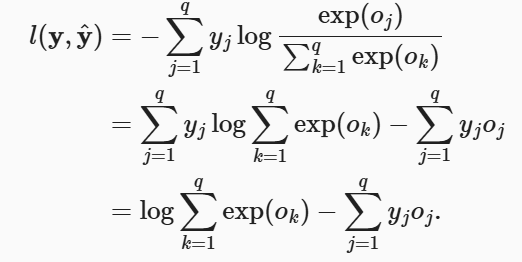
损失函数
使用最大似然估计:通常被称为交叉熵损失
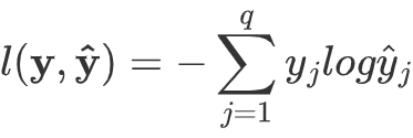
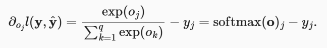
softmax导数分析:
(y1~q=1)
3.5 图像分类数据集
import:
1
2
3
4
5
6
import torch

from d2l import torch as d2l
from torch.utils import data
from torchvision import transforms
import torchvision
组件们
保存至d2l:
1
2
3
4
5
# 根据数字返回数据集的文本标签
def get_fashion_mnist_labels(labels):  # @save
    text_labels = ['t-shirt', 'trouser', 'pullover', 'dress', 'coat',
                   'sandal', 'shirt', 'sneaker', 'bag', 'ankle boot']
    return [text_labels[int(i)] for i in labels]
1
2
3
4
5
6
7
8
9
10
11
12
13
14
15
16
17
# 绘制图像列表
def show_images(imgs, num_rows, num_cols, titles=None, scale=1.5):  #@save
    figsize = (num_cols * scale, num_rows * scale)
    _, axes = d2l.plt.subplots(num_rows, num_cols, figsize=figsize)
    axes = axes.flatten()
    for i, (ax, img) in enumerate(zip(axes, imgs)):
        if torch.is_tensor(img):
            # 图片张量
            ax.imshow(img.numpy())
        else:
            # PIL图片
            ax.imshow(img)
        ax.axes.get_xaxis().set_visible(False)
        ax.axes.get_yaxis().set_visible(False)
        if titles:
            ax.set_title(titles[i])
    return axes
1
2
3
# 使用4个进程来读取数据
def get_dataloader_workers():  # @save
    return 4
简要流程:
下载并读取数据集
1
2
3
4
5
6
7
8
9
# ToTensor将图像数据从PIL类型变换成32位浮点数格式
# 并除以255使得所有像素的数值均在0到1
trans = transforms.ToTensor()
mnist_train = torchvision.datasets.FashionMNIST(
    root='../data', train=True, transform=trans, download=True
)
mnist_test = torchvision.datasets.FashionMNIST(
    root='../data', train=False, transform=trans, download=True
)
数据集的特征
1
2
3
4
print(len(mnist_train))
print(len(mnist_test))
# 每个输入图像的高度和宽度均为28像素,数据集由灰度图像组成,通道数为1
print(mnist_train[0][0].shape)
60000
10000
torch.Size([1, 28, 28])</br>训练数据集中取样并绘图
1
2
3
X, y = next(iter(data.DataLoader(mnist_train, batch_size=18)))
show_images(X.reshape(18, 28, 28), 2, 9, titles=get_fashion_mnist_labels(y));
d2l.plt.show()
打乱所有样本读取小批量
1
2
3
4
batch_size = 256

train_iter = data.DataLoader(mnist_train, batch_size, shuffle=True,
                             num_workers=get_dataloader_workers())
整合组件
保存至d2l:
1
2
3
4
5
6
7
8
9
10
11
12
13
14
def load_data_fashion_mnist(batch_size, resize=None):  # @save
    """下载Fashion-MNIST数据集,然后将其加载到内存中"""
    trans = [transforms.ToTensor()]
    if resize:
        trans.insert(0, transforms.Resize(resize))
    trans = transforms.Compose(trans)
    mnist_train = torchvision.datasets.FashionMNIST(
        root="../data", train=True, transform=trans, download=True)
    mnist_test = torchvision.datasets.FashionMNIST(
        root="../data", train=False, transform=trans, download=True)
    return (data.DataLoader(mnist_train, batch_size, shuffle=True,
                            num_workers=get_dataloader_workers()),
            data.DataLoader(mnist_test, batch_size, shuffle=False,
                            num_workers=get_dataloader_workers()))
指定resize参数来测试函数的图像大小调整功能:
1
2
3
4
5
if __name__ == "__main__":  # 多进程使用,确保只有主进程才会执行下面代码
    train_iter, test_iter = load_data_fashion_mnist(32, resize=64)
    for X, y in train_iter:
        print(X.shape, X.dtype, y.shape, y.dtype)
        break
torch.Size([32, 1, 64, 64]) torch.float32 torch.Size([32]) torch.int64
3.6 softmax回归的从零开始实现
import:
1
2
3
import torch
from IPython import display
from d2l import torch as d2l
保存至d2l
1
2
3
4
5
6
# 计算预测正确的数量
def accuracy(y_hat, y):  # @ save
    if len(y_hat.shape) > 1 and y_hat.shape[1] > 1:
        y_hat = y_hat.argmax(axis=1)
    cmp = y_hat.type(y.dtype) == y
    return float(cmp.type(y.dtype).sum())
1
2
3
4
5
6
7
8
9
def evaluate_accuracy(net, data_iter):  # @save
    """计算在指定数据集上模型的精度"""
    if isinstance(net, torch.nn.Module):
        net.eval()  # 将模型设置为评估模式
    metric = Accumulator(2)  # 正确预测数、预测总数
    with torch.no_grad():
        for X, y in data_iter:
            metric.add(accuracy(net(X), y), y.numel())
    return metric[0] / metric[1]
1
2
3
4
5
6
7
8
9
10
11
12
13
14
class Accumulator:  # @save
    """在n个变量上累加"""

    def __init__(self, n):
        self.data = [0.0] * n

    def add(self, *args):
        self.data = [a + float(b) for a, b in zip(self.data, args)]

    def reset(self):
        self.data = [0.0] * len(self.data)

    def __getitem__(self, idx):
        return self.data[idx]
1
2
3
4
5
6
7
8
9
10
11
12
13
14
15
16
17
18
19
20
21
22
23
def train_epoch_ch3(net, train_iter, loss, updater):  # @save
    """训练模型一个迭代周期(定义见第3章)"""
    # 将模型设置为训练模式
    if isinstance(net, torch.nn.Module):
        net.train()
    # 训练损失总和、训练准确度总和、样本数
    metric = Accumulator(3)
    for X, y in train_iter:
        # 计算梯度并更新参数
        y_hat = net(X)
        l = loss(y_hat, y)
        if isinstance(updater, torch.optim.Optimizer):
            # 使用PyTorch内置的优化器和损失函数
            updater.zero_grad()
            l.mean().backward()
            updater.step()
        else:
            # 使用定制的优化器和损失函数
            l.sum().backward()
            updater(X.shape[0])
        metric.add(float(l.sum()), accuracy(y_hat, y), y.numel())
    # 返回训练损失和训练精度
    return metric[0] / metric[2], metric[1] / metric[2]
1
2
3
4
5
6
7
8
9
10
11
12
13
14
15
16
17
18
class Animator:  # @save
    """在动画中绘制数据"""

    def __init__(self, xlabel=None, ylabel=None, legend=None, xlim=None,
                 ylim=None, xscale='linear', yscale='linear',
                 fmts=('-', 'm--', 'g-.', 'r:'), nrows=1, ncols=1,
                 figsize=(3.5, 2.5)):
        # 增量地绘制多条线
        if legend is None:
            legend = []
        d2l.use_svg_display()
        self.fig, self.axes = d2l.plt.subplots(nrows, ncols, figsize=figsize)
        if nrows * ncols == 1:
            self.axes = [self.axes, ]
        # 使用lambda函数捕获参数
        self.config_axes = lambda: d2l.set_axes(
            self.axes[0], xlabel, ylabel, xlim, ylim, xscale, yscale, legend)
        self.X, self.Y, self.fmts = None, None, fmts
1
2
3
4
5
6
7
8
9
10
11
12
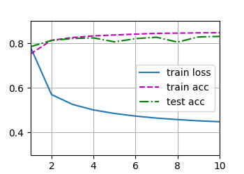
def train_ch3(net, train_iter, test_iter, loss, num_epochs, updater): # @save
"""训练模型(定义见第3章)"""
animator = Animator(xlabel='epoch', xlim=[1, num_epochs], ylim=[0.3, 0.9],
legend=['train loss', 'train acc', 'test acc'])
for epoch in range(num_epochs):
train_metrics = train_epoch_ch3(net, train_iter, loss, updater)
test_acc = evaluate_accuracy(net, test_iter)
animator.add(epoch + 1, train_metrics + (test_acc,))
train_loss, train_acc = train_metrics
assert train_loss < 0.5, train_loss
assert train_acc <= 1 and train_acc > 0.7, train_acc
assert test_acc <= 1 and test_acc > 0.7, test_acc
1
2
3
4
5
6
7
8
9
def predict_ch3(net, test_iter, n=6):  # @save
    """预测标签(定义见第3章)"""
    for X, y in test_iter:
        break
    trues = d2l.get_fashion_mnist_labels(y)
    preds = d2l.get_fashion_mnist_labels(net(X).argmax(axis=1))
    titles = [true + '\n' + pred for true, pred in zip(trues, preds)]
    d2l.show_images(
        X[0:n].reshape((n, 28, 28)), 1, n, titles=titles[0:n])
使用实例
1
2
3
4
5
6
7
8
9
10
11
12
13
14
15
16
17
18
19
20
21
22
23
24
25
if __name__ == '__main__':
    # 定义交叉熵损失函数
    y = torch.tensor([0, 1, 1])
    y_hat = torch.tensor([[0.5, 0.2, 0.3], [0.1, 0.4, 0.5], [0.6, 0.3, 0.1]])

    print(y_hat[[0, 1, 2], y])

    print(cross_entropy(y_hat, y))
    print(accuracy(y_hat, y) / len(y))

    # 使用随机权重初始化net模型,模型精度接近于随机猜测,这里为接近0.1
    print(evaluate_accuracy(net, test_iter))

    lr = 0.1

    def updater(batch_size):
        return d2l.sgd([w, b], lr, batch_size)


    num_epochs = 10
    train_ch3(net, train_iter, test_iter, cross_entropy, num_epochs, updater)


    predict_ch3(net, test_iter)
    d2l.plt.show()
输出结果
tensor([0.5000, 0.4000, 0.3000])
tensor([0.6931, 0.9163, 1.2040])
0.3333333333333333
0.1345
3.7 softmax回归的简洁实现
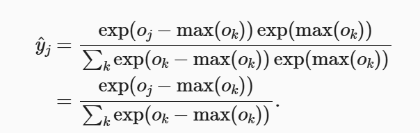
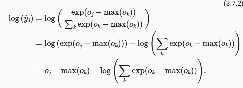
损失函数的数学原理
实现
1
2
3
4
5
6
7
8
9
10
11
12
13
14
15
import matplotlib.pyplot as plt
import torch
from torch import nn
from d2l import torch as d2l

batch_size = 256
train_iter, test_iter = d2l.load_data_fashion_mnist(batch_size)

net = nn.Sequential(nn.Flatten(), nn.Linear(784, 10))
loss = nn.CrossEntropyLoss(reduction='none')
trainer = torch.optim.SGD(net.parameters(),lr=0.1)

num_epochs = 10
d2l.train_ch3(net,train_iter,test_iter,loss,num_epochs,trainer)
plt.show()