02-预备知识
2.1 数据操作🎊
x = torch.arange(num) # 非额外指定,张量存储在内存,基于CPU计算x.shapex.numel() # 张量中元素的总数x.reshape(num1,num2,...)torch.zeros((num1,num2,num3,...))torch.ones((num1,num2,num3,...))torch.randn(num1,num2) # 从均值为0,标准差为1的正态分布(高斯分布)中随机采样torch.rand() # 包含从区间(0,1)均匀分布中抽取的一组随机数
x ** y # x的y次幂torch.exp(x)1 2 3 4
X = torch.arange(12, dtype=torch.float32).reshape((3, 4)) # shape:[3,4] Y = torch.tensor([[2, 1, 4, 3], [1, 2, 3, 4], [4, 3, 2, 1]]) # shape:[3,4] print(torch.cat((X, Y), dim=0)) # shape:[6,4] print(torch.cat((X, Y), dim=1)) # shape:[3,8]
X == YX.sum() # 对张量中所有元素进行求和
广播机制
1
2
3
4
5
[[0],                    [[0,0],    [[1,2],

 [1],  +  [[1,2]]  ---->  [1,1],  +  [1,2],

 [2]]                     [2,2]]     [1,2]]
索引和切片
X[-1],X[1:3]
可以写入
节省内存:执行原地操作
1
2
Z = torch.zeros_like(Y)
Z[:] = X + Y
1
X += Y  # 后续计算没有重复使用X的情况下
与其他python对象的转换
1
2
3
4
5
6
7
8
A = X.numpy()
B = torch.tensor(A)

print(type(A))
print(type(B))  # 共享底层内存,就地操作更改一个也会更改另一个

# <class 'numpy.ndarray'>
# <class 'torch.Tensor'>
2.2 数据预处理
数据集文件的创建与读取
1
2
3
4
5
6
7
8
9
10
import os

os.makedirs(os.path.join('..', 'data'), exist_ok=True)  # 在当前文件的上一级创建文件夹data
data_file = os.path.join('..', 'data', 'house_tiny.csv')  # 在文件夹data里面创建csv文件
with open(data_file, 'w') as f:
    f.write('NumRooms,Alley,Price\n')  # 列名
    f.write('NA,Pave,127500\n')  # 每行表示一个数据样本
    f.write('2,NA,106000\n')
    f.write('4,NA,178100\n')
    f.write('NA,NA,140000\n')
1
2
3
4
import pandas as pd

data = pd.read_csv(data_file)
print(data)
NumRooms Alley Price
0 NaN Pave 127500
1 2.0 NaN 106000
2 4.0 NaN 178100
3 NaN NaN 140000
处理缺失值
1 2 3 4 5
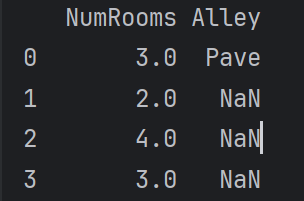
# inputs: data的前两列 # output: data的第三列 inputs, outputs = data.iloc[:, 0:2], data.iloc[:, 2] inputs = inputs.fillna(inputs.mean()) # 用同一列的均值填充缺少的数值 print(inputs) # 用均值填充后的inputs如下
1 2 3
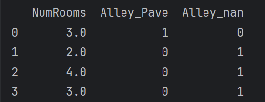
# 将非数值数据转为数值数据 inputs = pd.get_dummies(inputs, dummy_na=True) print(inputs) # 处理后的inputs如下
转换为张量格式
1 2 3 4 5
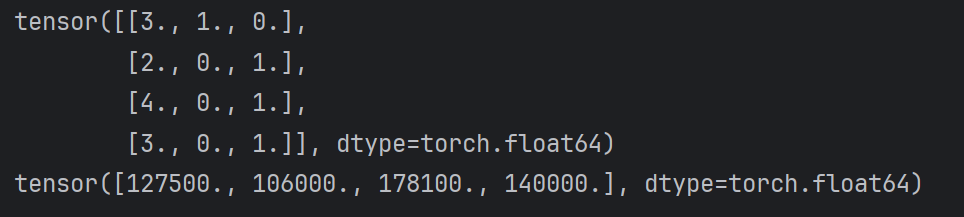
# 将数值数据转为张量 x = torch.tensor(inputs.to_numpy(dtype=float)) y = torch.tensor(outputs.to_numpy(dtype=float)) print(x) print(y)
2.3 线性代数
基本数学对象
- 标量:只有一个元素的张量,由小写字母表示
- 向量:通过一维张量表示,通常记为粗体、小写的符号
- 矩阵:在代码中表示为具有两个轴的张量,通常用粗体、大写字母来表示(行列数相同为方阵)
- 张量:描述具有任意数量轴的n维数组的通用方法,用特殊字体的大写字母表示(例如X, Y, Z)
张量算法的基本操作
1
2
A = torch.arange(20, dtype=torch.float32).reshape(5, 4)
B = A.clone()  # 通过分配新内存,将A的一个副本分配给B, B不随A变化
平均值
1
2
3
4
5
print(A.mean())
print(A.sum() / A.numel())

print(A.mean(axis=0))
print(A.sum(axis=0)/A.shape[0])
tensor(9.5000) tensor(9.5000) tensor([ 8., 9., 10., 11.]) tensor([ 8., 9., 10., 11.])
求和
降维求和
1
2
3
A_sum_axis0 = A.sum(axis=0)  # 沿axis=0方向压缩
print(A_sum_axis0)
print(A_sum_axis0.shape)
tensor([40., 45., 50., 55.]) torch.Size([4])
非降维求和
1
2
sum_A = A.sum(axis=0, keepdims=True)
print(sum_A)  # shape->[1,4]
tensor([[40., 45., 50., 55.]])
1
2
res = A.cumsum(axis=0)  # 沿方向累计求和
print(res)
tensor([[ 0., 1., 2., 3.], [ 4., 6., 8., 10.], [12., 15., 18., 21.], [24., 28., 32., 36.], [40., 45., 50., 55.]])
乘法
两个矩阵的按元素乘法(Hadamard积)
res.ij = A.ij * B.ij
1
A * B
两个向量的点积
xTy
1
torch.dot(x,y)
1
torch.sum(x * y)
矩阵-向量积
A.shape = [a,b]
x.shape = [b]
res.shape = [a]
1
torch.mv(A,x)
矩阵矩阵乘法(矩阵乘法)
1
torch.mm(A,B)
适用性最多的,能处理batch、广播的矩阵
1
torch.matmul(X,w) + b
范数
L2范数:常省略下标2
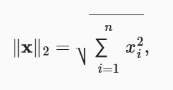
1
2
u = torch.tensor([3.0,-4.0])
torch.norm(u)  # 5
L1范数:受异常值的影响较小
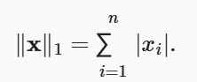
1
torch.abs(u).sum()  # 7
矩阵的Frobenius范数
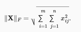
1
torch.norm(torch.ones((4,9)))  # 6
2.4 微积分
#@save进入d2l包内的函数
1
use_svg_display()  # 使用svg格式在Jupyter中显示绘图
1
set_figsize(figsize=(3.5, 2.5))  # 设置matplotlib的图表大小
1
set_axes(axes, xlabel, ylabel, xlim, ylim, xscale, yscale, legend)  # 设置matplotlib的轴
1
2
3
plot(X, Y=None, xlabel=None, ylabel=None, legend=None, xlim=None,
         ylim=None, xscale='linear', yscale='linear',
         fmts=('-', 'm--', 'g-.', 'r:'), figsize=(3.5, 2.5), axes=None)  # 绘制数据点
使用实例:
1
2
3
4
x = np.arange(0, 3, 0.1)
plot(x, [f(x), 2 * x - 3], 'x',
     legend=['f(x)', 'Tangent line (x = 1)'])
plt.show()
2.5 自动微分
x = torch.arange(4.0, requires_grad=True) #PyTorch只允许浮点类型和负数类型的张量在计算图中进行梯度运算(float,complex)
标量变量的反向传播
y = 2 *xTx
y = 2 * torch.dot(x, x)
1
2
y.backward()
print(x.grad)
tensor([ 0., 4., 8., 12.])
1
2
3
4
x.grad.zero_()  # 默认情况会累计梯度,如果不清空结果为[1,5,9,13]
y = x.sum()
y.backward()
print(x.grad)
tensor([1., 1., 1., 1.])
非标量变量的反向传播
1
2
3
4
5
x.grad.zero_()
y = x * x
y.sum().backward()
# 等价于y.backward(torch.ones(len(x)))
print(x.grad)
tensor([0., 2., 4., 6.])
注:两个等价
个人理解,y.sum().backward(), 将xi的平方求和反向传播,关于xi的导数只与自身有关与其他x值无关,求和能够满足分别求导的目的,不求和无法确定求导的形状;
y.backward(torch.ones(len(x))),显式地传递了一个全为1的张量作为权重,且形状与y相同。
1
2
3
4
x.grad.zero_()
y = x * x
y.backward(torch.tensor([1, 2, 4, 3]))  # 设置权重
print(x.grad)
tensor([ 0., 4., 16., 18.])
分离计算
1
2
3
4
5
6
7
8
x.grad.zero_()
y = x * x
u = y.detach()  # u与y具有完全相同的值,但是梯度不会向后流经y到x
z = u * x

z.sum().backward()  # 求导把u作为常数
print(x.grad == u)
print(x.grad == y)  # 输出均为True
2.6 概率
使用实例
1
2
3
4
5
6
7
# 概率向量
fair_probs = torch.ones([6]) / 6
# 进行total_count次实验
# .sample() 进行采样
sample = multinomial.Multinomial(1, fair_probs).sample()
samples = multinomial.Multinomial(10, fair_probs).sample()
counts = multinomial.Multinomial(1000, fair_probs).sample()
绘图
1
2
3
4
5
6
7
8
9
10
11
12
13
counts = multinomial.Multinomial(10, fair_probs).sample((5,))
cum_counts = counts.cumsum(dim=0)
estimates = cum_counts / cum_counts.sum(dim=1, keepdim=True)

d2l.set_figsize((6, 4.5))
for i in range(6):
    d2l.plt.plot(estimates[:, i].numpy(),
                 label=("P(die=" + str(i + 1) + ")"))
d2l.plt.axhline(y=0.167, color='black', linestyle='dashed')  # 在当前图中绘制一条y=0.167的水平虚线
d2l.plt.gca().set_xlabel('Groups of experiments')
d2l.plt.gca().set_ylabel('Estimated probability')
d2l.plt.legend()  # 在图中显示图例,即在绘图时给不同元素指定的标签
d2l.plt.show()
一些概念
联合概率:P(A = a, B = b)
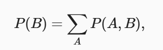
边际化:其结果的概率或分布称为边际概率或边际分布